.
S12 Sampling distributions
September 16, 2021 - 12:32pm — AJ (e67821)
A sampling distribution is the probability distribution for the means of all samples of size \(n\) from a given population.
The sampling distribution will be normally distributed with parameters \(\mu_{\overline{x}}\) and \(\sigma_{\overline{x}}\), if either:
the population from which the samples are drawn is normally distributed, or
the samples are large \((n\geqq30)\).
The mean of the sampling distribution (i.e. the mean of all the sample means, \(\mu\) \(_{\overline{x}}\)) and the standard deviation of the distribution (\(\sigma_{\overline{x}}\)) are given by:
\[ \mu_{\overline{x}}=\mu\quad and\quad\sigma_{\overline{x}}=\frac{\sigma}{\sqrt{n}} \] Note that:
The sampling distribution has the same centre as the population.
The measure of variability of a sampling distribution, \(\sigma_{\overline{x}}\), is called the standard error.
The distribution of means is not as spread out as the values in the population from which the sample was drawn.
If we do not know the population standard deviation we approximate with the sample standard deviation: \(s_{\overline{x}}\) \(\thickapprox\) \(\sigma_{\overline{x}}\) and \(\dfrac{s}{\sqrt{n}}\) \(\thickapprox\) \(\dfrac{\sigma}{\sqrt{n}}\) if the sample is large.
Example of a Sampling Distribution
Consider the little ‘population’ of values P = {1 2 3 4 5}
This population has \(\mu=3\) and \(\sigma=1.41\) .
If a sample of size n = 3 was drawn from this population it could be any one of:
(1 2 3) (1 2 4) (1 2 5) (1 3 4) (1 3 5) (1 4 5) (2 3 4) (2 3 5)
(2 4 5) (3 4 5)
The means of each of the samples, and a histogram of the distribution of means, are shown in the table and graph below:
| Sample | Mean |
|---|---|
| 1 2 3 | \(\overline{x}\) = 2 |
| 1 2 4 | \(\overline{x}\) = 2.33 |
| 1 2 5 | \(\overline{x}\) = 2.67 |
| 1 3 4 | \(\overline{x}\) = 2.67 |
| 1 3 5 | \(\overline{x}\) = 3 |
| 1 4 5 | \(\overline{x}\) = 3.33 |
| 2 3 4 | \(\overline{x}\) = 3 |
| 2 3 5 | \(\overline{x}\) = 3.33 |
| 2 4 5 | \(\overline{x}\) = 3.67 |
| 3 4 5 | \(\overline{x}\) = 4 |
\(\overline{\overline{x}}\) = 3 and \(\sigma_{\overline{x}}\) = 0.61
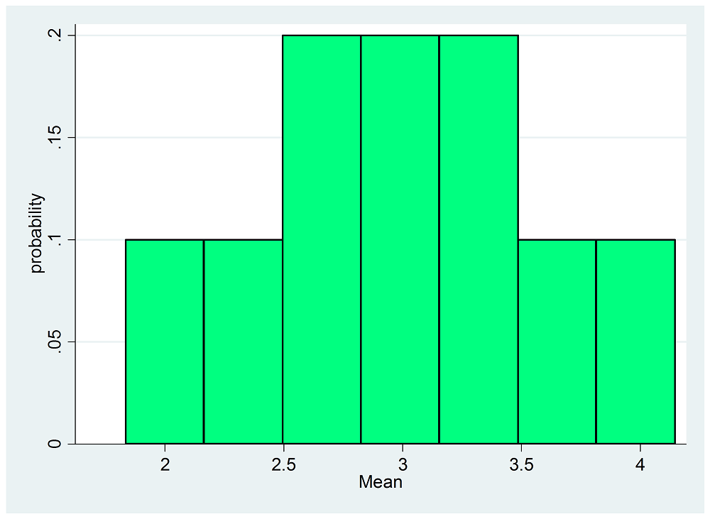
The sampling distribution of the means for samples of size 3 is:
| \(\overline{x}\) | 2 | 2.33 | 2.67 | 3 | 3.33 | 3.67 | 4 |
|---|---|---|---|---|---|---|---|
| P(\(\overline{X}=\overline{x}\)) | 0.1 | 0.1 | 0.2 | 0.2 | 0.2 | 0.1 | 0.1 |
Even though this sample is small, and the population is not normally distributed (though it is symmetric) the sampling distribution is reasonably normally distributed:
We can see that the mean of the sampling distribution (the mean of all the means) is the same as the population mean, \(\overline{\overline{x}}=\mu=3\). But the variability in the sampling distribution is less than that of the population: \(\sigma_{\overline{x}}=0.61\) and \(\sigma=1.41\). Because larger samples, or those drawn from normally distributed populations, will follow a normal distribution we can use the properties of normal distributions to find probabilities relating to samples: \[ z_{\overline{x}}=\dfrac{(\overline{x}-\mu)}{\sigma_{\overline{x}}}=\dfrac{(\overline{x}-\mu)}{\sigma/\sqrt{n}}. \]
Another Example
The shire of Bondara has 1200 preschoolers. The mean weight of pre-schoolers is known to be 18kg with a standard deviation of 3kg. What is the probability that a random sample of 50 preschoolers will have a mean weight more than 19kg?
\(n=50\), \(\mu=18\) and \(\sigma=3\)
The sampling distribution of the means for samples of size 50 will have \(\mu\) \(_{\overline{x}}\) \(=\) \(\mu=18\), and standard error, \[ \sigma_{\overline{x}}=\dfrac{\sigma}{\sqrt{n}}=\dfrac{3}{\sqrt{50}}=0.42 \] .
\[\begin{align*} z_{\overline{x}} & =\dfrac{(\overline{x}-\mu)}{\sigma/\sqrt{n}}\\ & =\dfrac{(19-18)}{3/\sqrt{50}}\\ & =2.38\\ \\ Pr(\overline{x}>19) & =Pr(z_{\overline{x}}>2.38)\\ & =1-0.9913\qquad[from\;tables]\\ & =0.0087 \end{align*}\]
Exercise
1. List all samples of size 2 for the population \({1,2,3,4,5,6}\). What is the probability of obtaining a sample mean of less than \(3\)?
\(4/15\)
2. Samples of size \(40\) are drawn from a population with \(\mu=50\) and \(\sigma=5\). What are the mean and standard error of the sampling distribution? What is the probability that a particular sample has a mean less than \(48.5\)?
(a) \(\mu\) \(_{\overline{x}}=50\) and \(\sigma_{\overline{x}}=0.79\quad\quad\)(b) \(0.0288\)
3. If IQ in the general population of secondary students is known to follow a normal distribution with \(\mu=100\) and \(\sigma=10\), find the mean and standard error for a random sample of size \(100\). To test whether a secondary school is representative of the general population a sample of \(100\) students from that school is chosen. What is the probability of the mean IQ being more than \(105\)? What would be your conclusion?
(a) \(\mu\) \(_{\overline{x}}=100\) and \(\sigma_{\overline{x}}=1\qquad\)(b) \(0.00003\thickapprox0\). This implies that either the sample was not random (perhaps all the smartest students were in the sample) or this school has a higher average IQ than the general population.
Download this page: S12 Sampling Distributions (PDF 168KB)
What's next... S13 Confidence intervals