.
S14 Hypothesis testing
September 16, 2021 - 12:33pm — AJ (e67821)
Consider statements such as
Teenagers aged \(13\)-\(15\) spend no more than \(10\) hours a week on Facebook.
The average weight of Australian men is the same as it was in \(1990\).
Students from private schools have the same mean ATAR score as the Victorian average.
The mean winter rainfall for the last \(10\) years is the same as the historical mean.
Our confidence about the probabilities of values drawn from normally distributed populations and sampling distributions enables us to formally test hypotheses (or claims) such as these.
When we perform an ‘experiment’ we know there will be chance variation. For example, if we toss a supposedly fair coin \(100\) times we would not be surprised to obtain \(48\) or \(45\) or perhaps even \(40\) heads. However we would be surprised to obtain only \(5\) heads. If we were testing a coin for ‘fairness’ we might decide beforehand what we would consider a reasonable number of heads. In hypothesis testing ‘reasonable’ is defined as what we could expect \(95\)% (or \(99\)% or \(90\)% etc) of the time.
In a hypothesis test we are concerned to assess how unusual our result is, whether it is reasonable chance variation (obtaining \(45\) heads in \(100\) tosses of a coin) or whether the result is too extreme to be considered chance variation (obtaining \(5\) heads in \(100\) tosses of a coin).
A hypothesis test formalizes the process of deciding whether a result is reasonable.
Steps in a Hypothesis Test
The steps are:
State the null and alternative hypotheses
\(H_{o}:\) \(\overline{x}=\mu\) (the sample mean is the same as the population mean after allowing for chance variation)
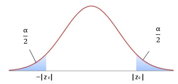
\(H_{a}:\overline{x}\neq\mu\) (the sample mean is not the same as the population mean after allowing for chance variation)Significance level \(\alpha\) is chosen (\(\alpha=0.05\Rightarrow\) we are defining reasonable as what we can expect 95% of the time)
Critical values
Tables or a calculator or a computer are used to find the z-values that corresponds to the chosen significance level. These are called the critical values.
Calculate the test statistic.
This is the standardised difference between the sample mean (calculated from the given data) and the known population mean: \[\begin{align*} z & =\frac{\overline{x}-\mu}{\frac{\sigma}{\sqrt{n}}}. \end{align*}\]Decision: Is the result reasonable if \(H_{o}\) is true?
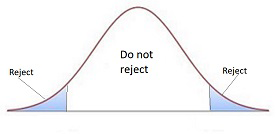
Is the test statistic more extreme than the critical value?
Yes \(\Rightarrow\) Reject \(H_{o},\) No \(\Rightarrow\) Do not reject \(H_{o}\).Conclusion
There is (if you reject)/is not (if you do not reject) evidence to suggest that… (Paraphrase the information in the question to complete the conclusion).
It is important to note that
- The decision about the null hypothesis is not made with certainty but with a level of confidence that the error in the decision is small (for example 5% if \(\alpha=0.05\))
- The decision relates only to rejecting or not rejecting \(H_{o}\). \(H_{a}\) is not mentioned in the decision, and we DO NOT ACCEPT \(H_{o}\) or \(H_{a}\)
- The steps for hypothesis testing may differ from course to course so check with your program.
Example
Because students had previously found a statistics course very difficult the average score over many years was \(48\)% with a standard deviation of \(12\)%. A bridging program was introduced and the \(120\) students that attended achieved a mean score of \(50\)% in the final exam. Is there evidence that the scores of those who attended the bridging program have changed at a \(1\)% level of significance?
State the hypotheses
\(H_{o}:\) \(\overline{x}=48\) (the sample mean is the same as the population mean)
\(H_{a}:\overline{x}\neq48\) (the sample mean is not the same as the population mean)Significance level \(\alpha=0.01\)
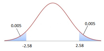
Critical values
\(\alpha=0.01\) \(\Rightarrow z=-2.58\textrm{ or }\) \(z=2.58\)
Test statistic
\[\begin{align*} z & =\frac{\overline{x}-\mu}{\frac{\sigma}{\sqrt{n}}}\\ & =\frac{50-48}{\frac{12}{\sqrt{120}}}\\ & =1.83. \end{align*}\]Decision:
Is \(1.83\) more extreme than \(2.58?\) No \(\Rightarrow\) Do not reject \(H_{o}\)Conclusion
There is not enough evidence to suggest that the scores of those who attended the bridging program have changed.
(It is reasonable that the apparent improvement is due to chance variation).
Exercises
Your answers should be set out and contain all the steps shown above. A brief outline of the main features is given in the answers to teh following exercises.
1. Repeat the example to decide if there is evidence at the \(10\)% level of significance that attending the bridging program is associated with the change in scores.
Test statistic \(=1.83\) reject \(H_{o}\): evidence of change in scores.
2. A random sample of \(36\) soft drinks from vending machines had an average content of \(370\)ml with a standard deviation of \(20\)ml. Test the null hypothesis that \(\mu\) \(=375\) ml against the alternative hypothesis \(\mu\) \(\neq375\)ml at the \(1\)% significance level.
Test statistic \(=-1.5\) do not reject \(H_{o}\): difference consistent with chance variation
3. A bank manager has historical data that shows over lunchtime Mon – Fri the mean number of customers that come into the bank is \(32\). Accordingly he believes he has no need to change the number of tellers. However a branch survey conducted every lunchtime over eight weeks found that the mean number of customers was \(36\) with a standard deviation of \(8.2\). Conduct a hypothesis test with a \(5\)% level of significance to test whether the mean number of lunchtime customers has changed. What recommendation would you make to the bank manager?
Test statistic \(=3.09\) reject \(H_{o}\): evidence of increase in lunchtime customers, therefore need more tellers
4. The manufacturer of ‘longlast’ batteries claims the mean lifetime of his batteries is \(450\) hours. A consumer interest magazine samples 100 batteries and finds that they have a mean of \(444\) hours with a standard deviation of \(28\) hours. Do the sample data contradict the manufacturers claim? (use \(\alpha\) \(=0.02\))
Test statistic \(=2.14\) do not reject \(H_{o}\): the difference is consistent with chance variation and there is no evidence to contradict the claim that the mean battery life is \(450\) hours.
Download this page: S14_Hypothesis_Testing (PDF 1.907KB)
What's next... S15 T-test