.
FG9 Graphs and transformations
August 11, 2022 - 2:30pm — AJ (e67821)
The known graphs of some simple functions and relations can be used to sketch related, but more complicated functions.
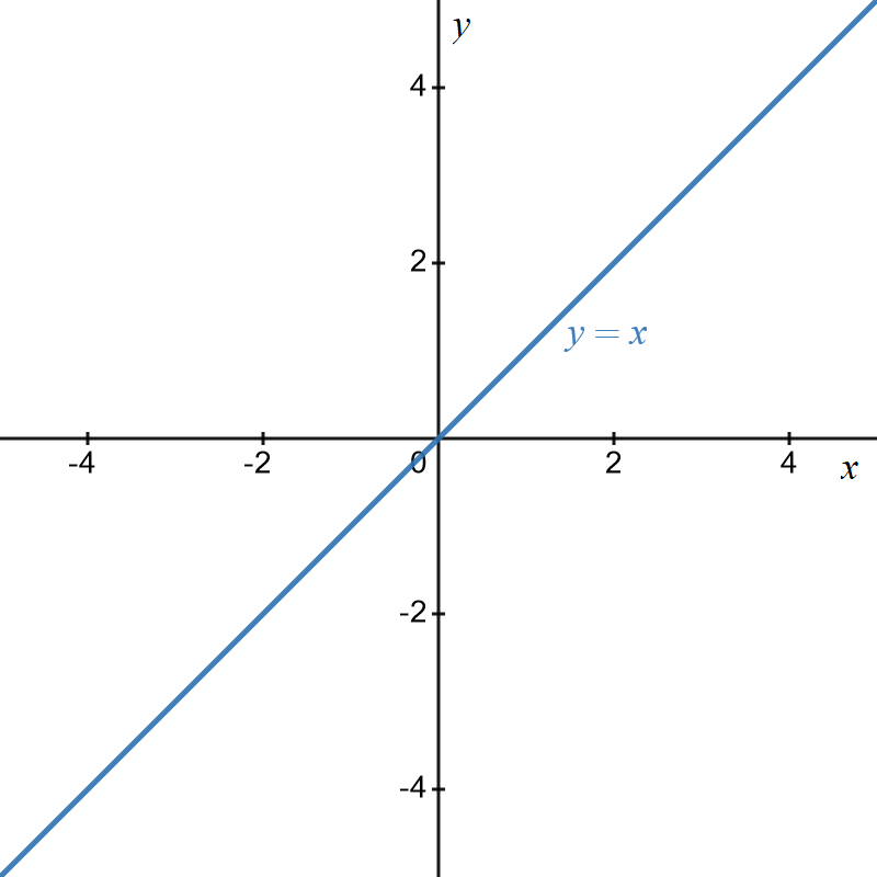
If you know the graph of a function, you can often transform it to a graph of a more complex but related function. A simple example is the graph of the line \[\begin{align*} y & =x. \end{align*}\] It has the graph:
The graph of \[\begin{align*} y & =x+2 \end{align*}\] is shown in red below
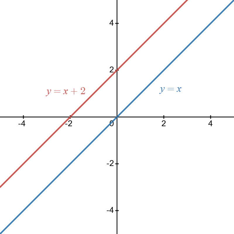
This is just the graph of \(y=x\) shifted \(2\) units upward and is an example of a transformation involving vertical translation.
This module discusses how to transform the graphs of known functions to more complex functions using simple rules that are called transformations. In particular, we will consider the following transformations:
Reflection
Translation
Dilation
Combinations of the above.
Basic Graphs
When attempting to graph a function, the following items need to be considered:
\(x\) and \(y\) intercepts
turning points
behavior as \(x\rightarrow\pm\infty\)
asymptotes. It is very useful to know the graphs of some simple functions. You can then transform them to more complex functions using the contents of this module. Below are some basic graphs that you should know.1 While it is best that you know these graphs, if you cannot recall them, you can still determine their graphs by plotting some points.
Graph of \(y=x\)
This is a straight line with slope or gradient of \(1.\) It passes through the origin and is shown below.
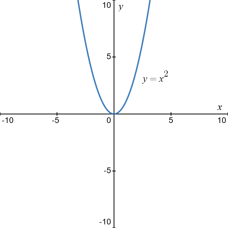
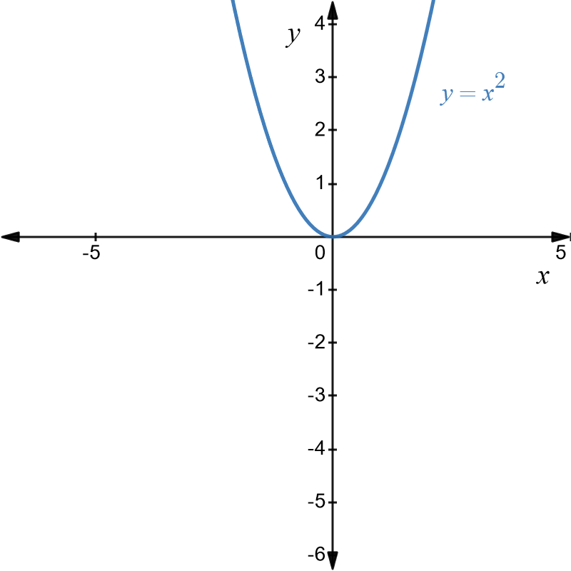
Graph of \(y=x^{2}\)
This is a parabola with vertex at the origin as shown below.
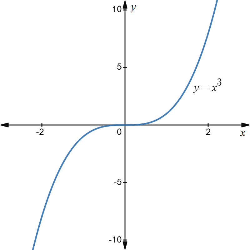
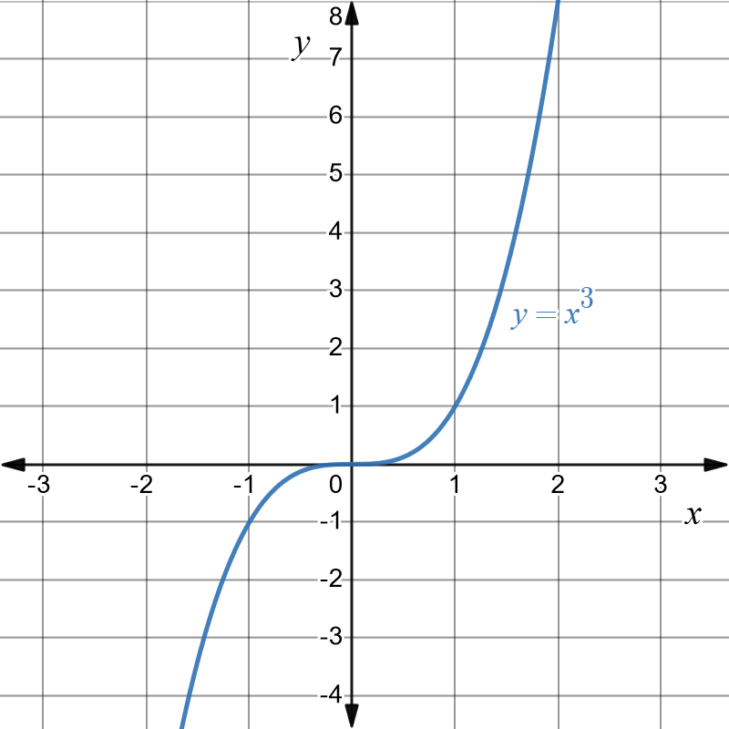
Graph of \(y=x^{3}\)
The essential feature is that the graph goes through the origin increases for positive \(x\) and decreases for negative \(x.\)
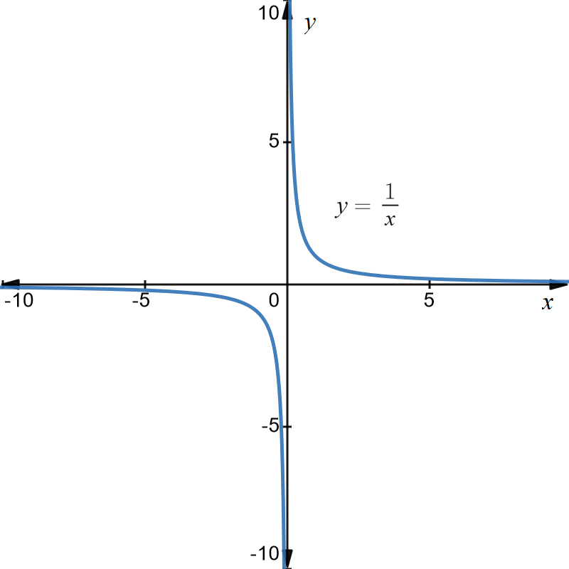
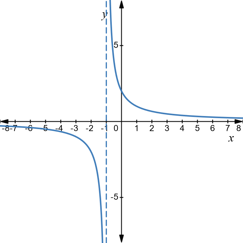
Graph of \(y=1/x\)
This is a graph with asymptotes at \(x=0\) and \(y=0\) (the \(x-\) axis) as shown below.
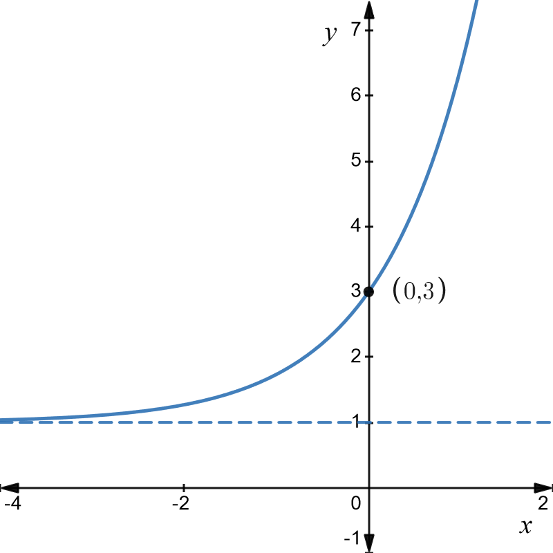
Graph of \(y=a^{x}\)
The basic graph is as shown below for \(a=1.6\).
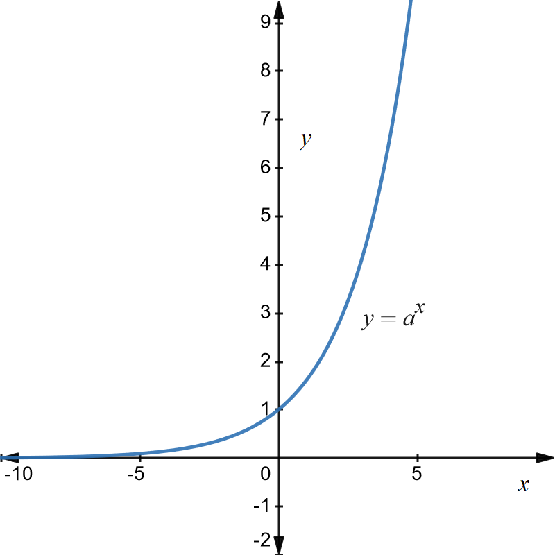
The important thing to note is that the \(y-\) intercept is at \(1\) and doesn’t depend on the value of \(a\) because \(a^{0}=1.\) Also the function cannot be less than zero so the negative \(x-\)axis is an asymptote. Changing the value of \(a\) will change the values on the \(y-\)axis but the basic shape of the graph is the same. In practice, the most common value of \(a\) is \(e\) and is most likely to come up in your course. So the graph above gives the basic shape of \(y=e^{x}\) but the \(y-\) axis values are incorrect.
Graph of \(y=\log x\)
The graph is shown below.
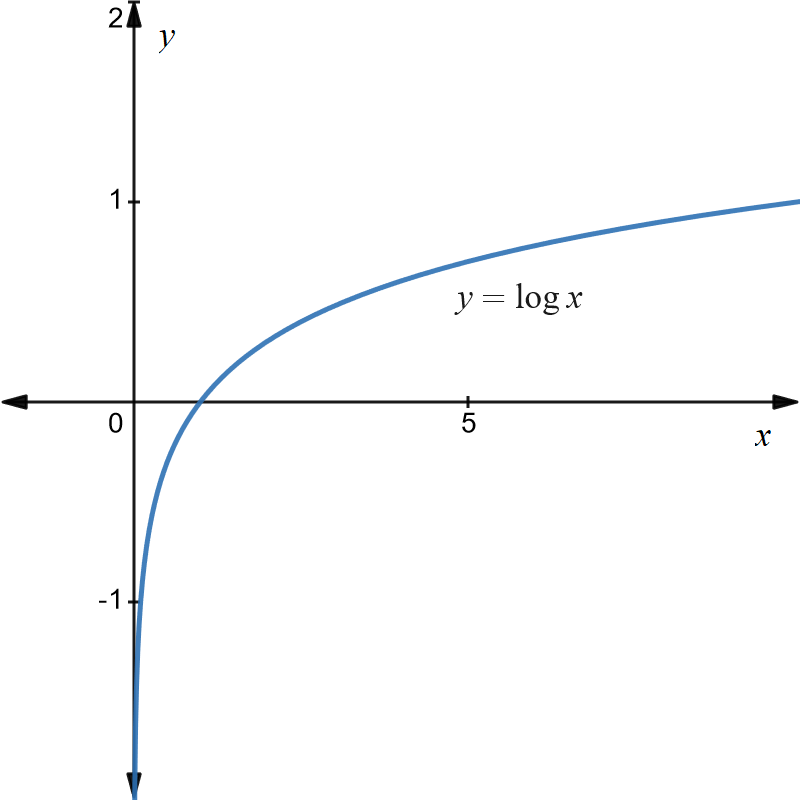
The important characteristic is that the graph cuts the \(x-\) axis at \(1\) because \(\log\left(1\right)=0.\) Note that this graph is similar for \(\ln\left(x\right)=\log_{e}\left(x\right)\) or any other log base .
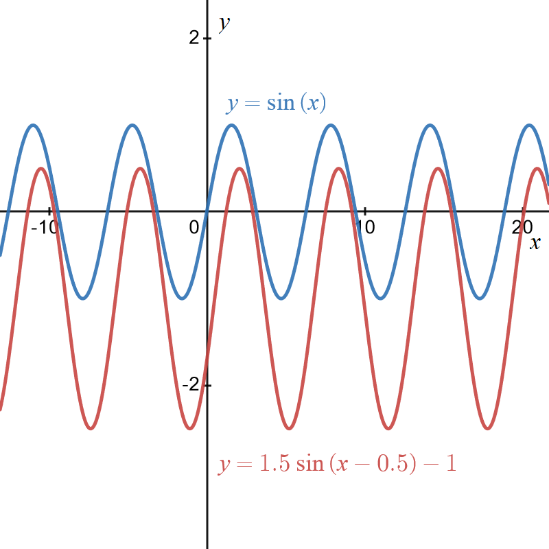
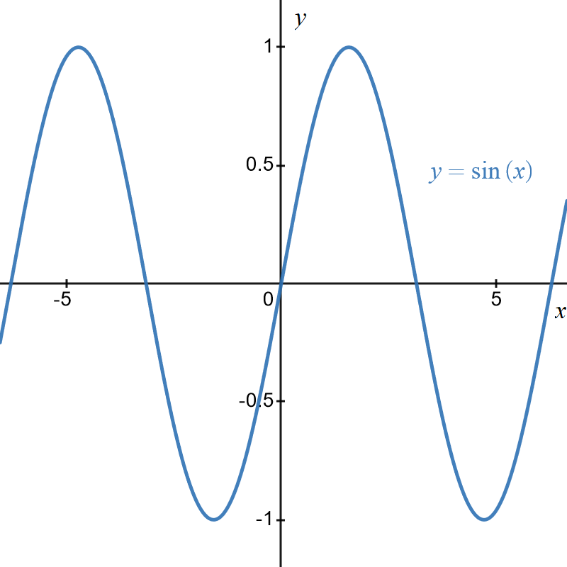
Graph of \(y=\sin\left(x\right)\)
Transformations
As mentioned above, transformations may be used to modify basic graphs. The transformations are
Reflection
Translation
Dilation
Combinations of the above.
Reflection
As the name suggests, a reflection is a mirror image of a graph. Reflection may be about any line but generally involves the \(x\) or \(y\) axes.
For a graph \(y=f\left(x\right),\) \[\begin{align*} y & =f\left(-x\right) \end{align*}\] reflects the graph about the \(y-\)axis while
\[\begin{align*} y= & -f\left(x\right) \end{align*}\] reflects the graph about the \(x-\)axis.
Example \(1\): Reflection of \(y=a^{x}\) in the \(x\) and \(y\) axes
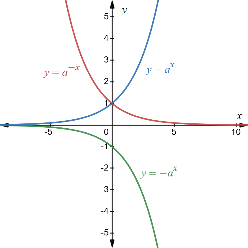
Referring to the graphs shown below.
The original graph is \(y=a^{x}\) and is shown in blue.
Reflection about the \(y-\)axis is given by \(y=a^{-x}\) and is shown in red.
Reflection about the \(x-\)axis is given by \(y=-a^{x}\) and is shown in green.
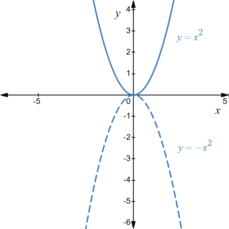
Example \(2\): Reflection of \(y=x^{2}\) in the \(x\) and \(y\) axes
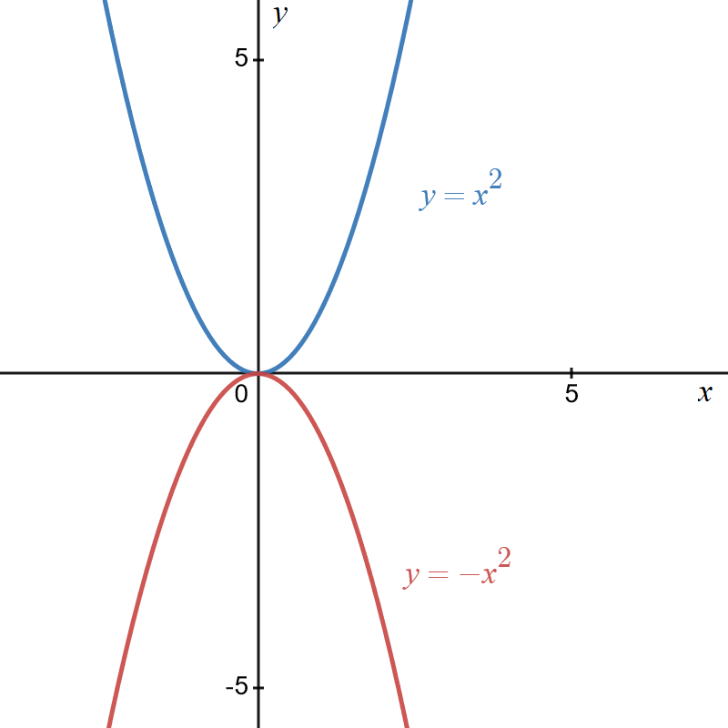
Original graph is \(y=x^{2}\) and is shown in blue below
Reflection about the \(y-\)axis is given by \(y=\left(-x\right)^{2}=x^{2}.\) This means the reflection in the \(y-\)axis of the original graph doesn’t change anything. This is due to symmetry of the original graph about the \(y-\)axis.
Reflection about the \(x-\)axis is given by \(y=-x^{2}\) and is shown below in red.
Example \(3\): Reflection of \(y=2x+1\) in the \(x\) and \(y\) axes
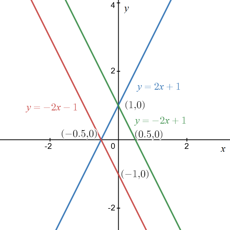
Original graph is \(y=2x+1\) and is shown in blue below.
Reflection in the \(y-\)axis is given by \(y=2\left(-x\right)+1=-2x+1\) and is shown in green.
Reflection in the \(x-\)axis is given by \(y=-\left(2x+1\right)=-2x-1\) and is shown in red.
Translation
Translation involves moving a graph, in the \(x-y\) plane, horizontally or vertically.
Horizontal
The graph of \(y=f\left(x-a\right)\) is a shift of the graph of \(y=f\left(x\right)\) “\(a\)” units to the right.
The graph of \(y=f\left(x+a\right)\) is a shift of the graph of \(y=f\left(x\right)\) “\(a\)” units to the left.
Vertical
The graph of \(y=f\left(x\right)+b\) is a shift of the graph of \(y=f\left(x\right)\) “\(b\)” units up.
The graph of \(y=f\left(x\right)-b\) is a shift of the graph of \(y=f\left(x\right)\) “\(b\)” units down.
Example \(4\): Translation of \(y=\log\left(x\right)\) \(1\) unit to the right.
Original graph is \(y=\log\left(x\right)\) and is shown in blue below. The translated graph is \(y=\log\left(x-1\right)\) and is shown in red below. It is the graph of the original function shifted \(1\) unit to the right.
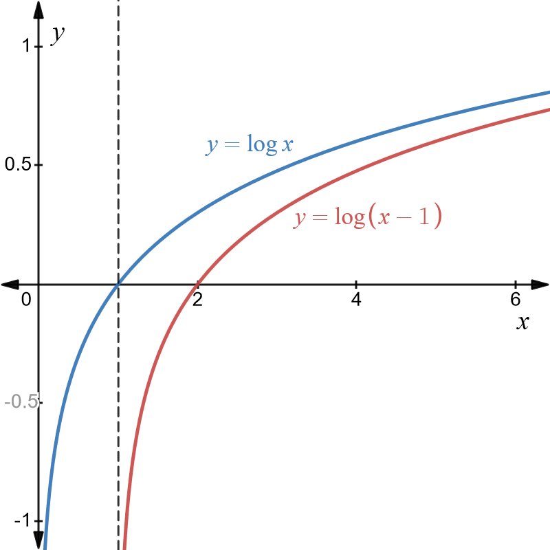
Note that the negative \(y-\)axis forms an asymptote for the original graph. The translated graph has an asymptote of \(x=1\) and is shown as a dotted line. The new asymptote should be shown on the graph of the transformed function.
Example \(5\): Translation of \(y=1/x\) three units to the left
The original graph is of \(y=1/x\) and is shown in blue below. The translated graph is \[\begin{align*} y & =\frac{1}{x+3} \end{align*}\] and is the graph of the original function shifted \(3\) units to the left. It is shown in red below.
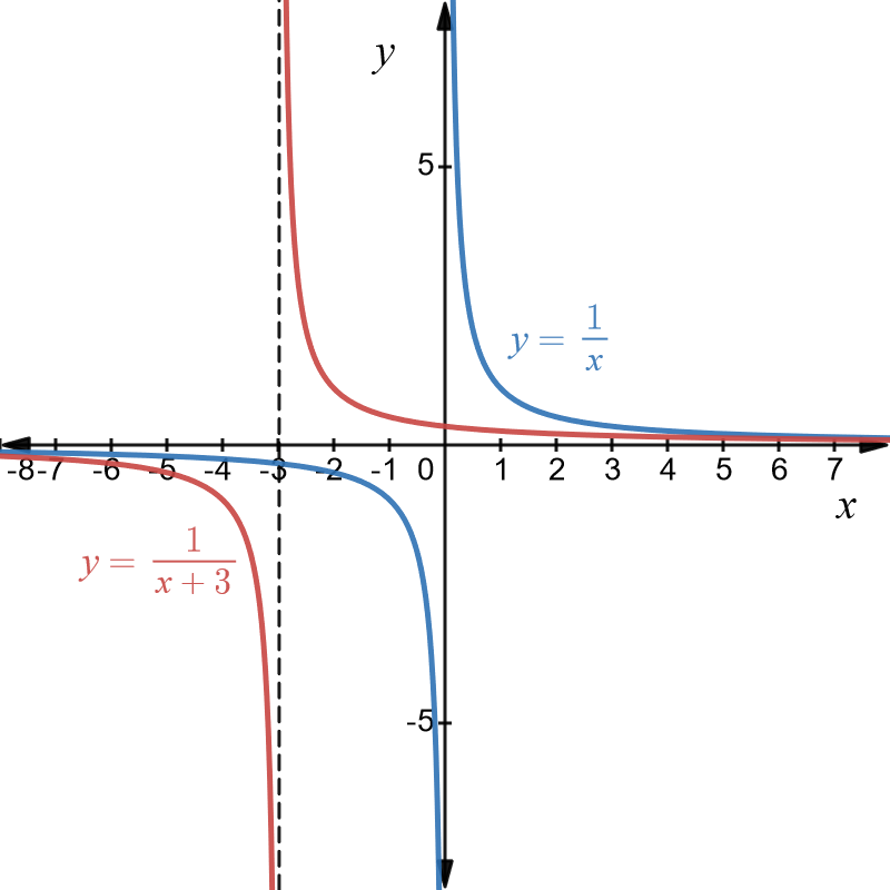
The original graph had the \(y-\)axis as its asymptote. The transformed graph has an asymptote at \(x=-1\) which is shown as a dotted line.
Example \(6\): Translation of \(y=\sin\left(x\right),\) \(\pi/2\) units to the left
The original graph is of \(y=\sin\left(x\right)\). The transformed graph is \(y=\sin\left(x+\pi/2\right)\) . Both graphs are shown below in blue and red respectively below.
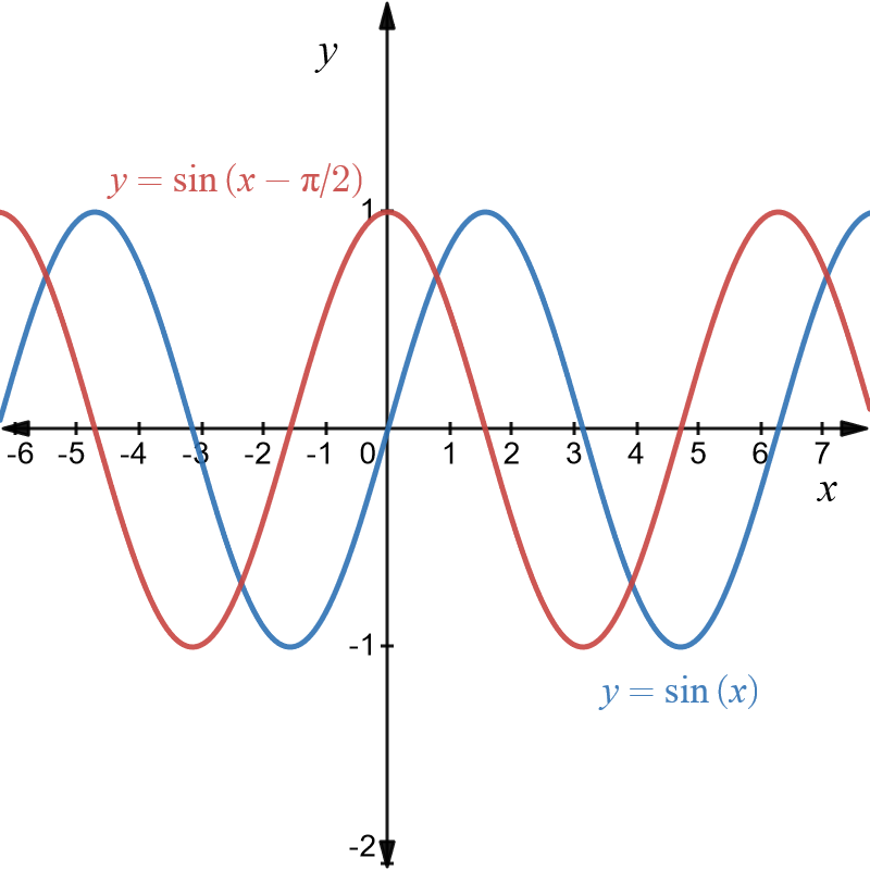
This is an interesting example as the translation converts the sine function to the cosine function.2 To see this, recall the trigonometry identity \[\begin{align*} \sin\left(a+b\right) & =\sin\left(a\right)\cos\left(b\right)+\cos\left(a\right)\sin\left(b\right). \end{align*}\] Now let \(a=x\) and \(b=\pi/2.\) Substituting in the above identity we get \[\begin{align*} \sin\left(x+\frac{\pi}{2}\right) & =\sin\left(x\right)\cos\left(\frac{\pi}{2}\right)+\cos\left(x\right)\sin\left(\frac{\pi}{2}\right)\\ & =\sin\left(x\right)\cdot0+\cos\left(x\right)\cdot1\\ & =\cos\left(x\right). \end{align*}\]
Example \(7\): Translation of \(y=\sin\left(x\right)\) two units vertically up
The original graph is of \(y=\sin\left(x\right)\). The transformed graph is \(y=\sin\left(x\right)+2\) . Both graphs are shown below in blue and red respectively below.
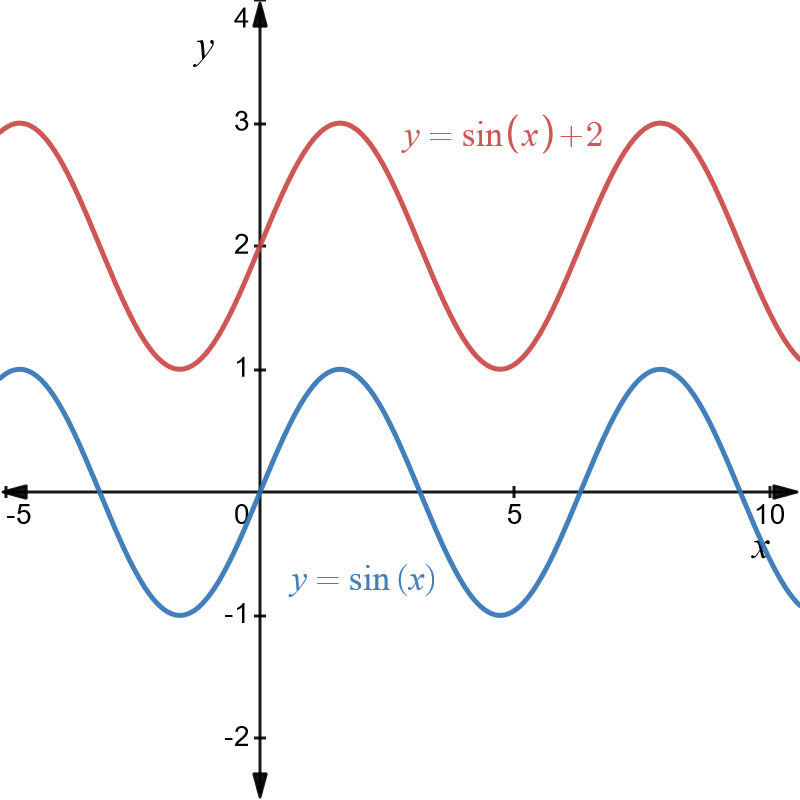
It is clear that the translation simply moves the graph of \(y=\sin\left(x\right)\) up \(2\) units. Nothing else changes.
Example \(8\): Translation of \(y=x^{2}\) two units vertically down
The original graph is of \(y=x^{2}\). The transformed graph is \(y=x^{2}-2\) . Both graphs are shown below in blue and red respectively.
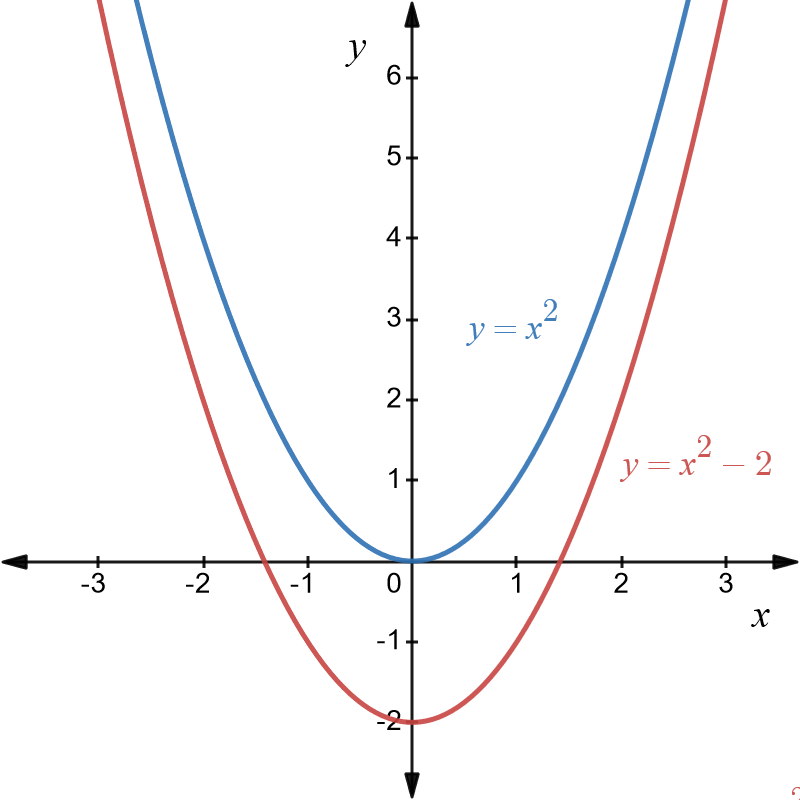
It is clear that the translation simply moves the graph of \(y=x^{2}\) down \(2\) units. Nothing else changes.
Dilations
Dilations stretch or compress a graph of a function. The stretching or compression can occur in the directions of either the \(x\) or the \(y\) axes, or both.
The graph of \(y=af\left(x\right)\) is a dilation of the graph of \(y=f\left(x\right)\) by a factor of “\(a\)” units in the direction parallel to the \(y-\)axis. If \(a>1\) the graph is stretched or elongated. If \(a<1,\)the graph is compressed or squashed.
The graph of \(y=f\left(bx\right)\) is a dilation of the graph of \(y=f\left(x\right)\) by a factor of “\(1/b\)” units in the direction parallel to the \(x-\)axis. If \(b>1\) the graph is compressed or squashed. If \(b<1,\)the graph is stretched or elongated.
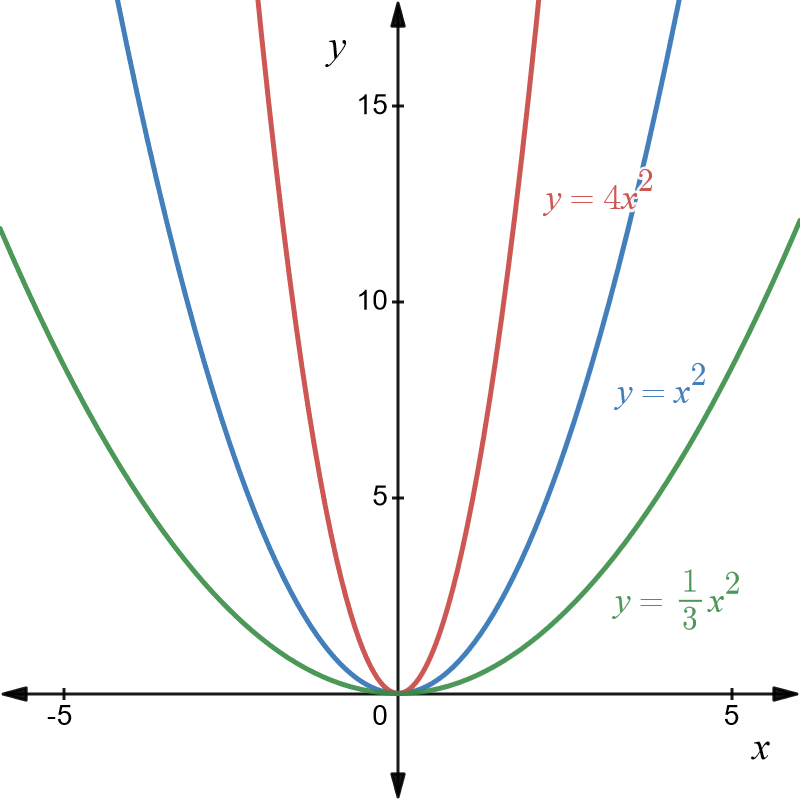
Example \(9\): Dilation of \(y=x^{2}\) parallel to the \(y-\)axis by a factor of \(4\) and 1/3
The graphs are shown below.
The original graph of \(y=x^{2}\) is shown in blue.
The dilation \(y=4x^{2}\) is shown in red and shows that the original graph is stretched parallel to the \(y-\) axis.
The dilation \(y=\frac{1}{3}x^{2}\)is shown in green and shows that the original graph is squashed parallel to the \(y-\) axis.
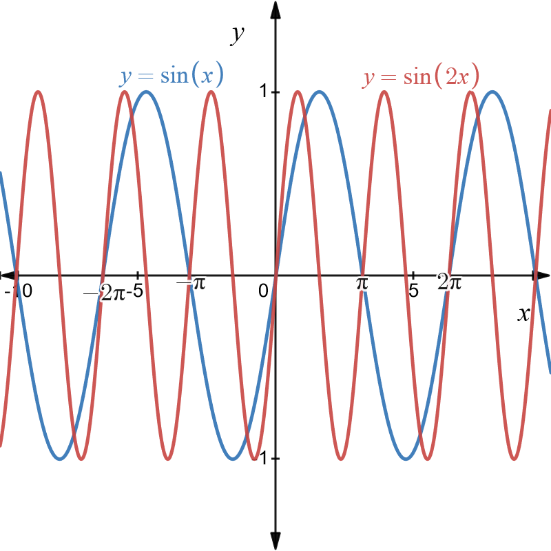
Example \(10\): Dilation of \(y=\sin\left(x\right)\) parallel to the \(x-\)axis by a factor of \(2\)
The graphs are shown below.
The original graph of \(y=\sin\left(x\right)\) is shown in blue. It has a period of \(2\pi.\)
The dilation \(y=\sin\left(2x\right)\) is shown in red and shows that the original graph is squashed by a factor of \(2\) parallel to the \(x-\) axis. The dilated graph has a period of \(\pi\) which is half that of the original graph.
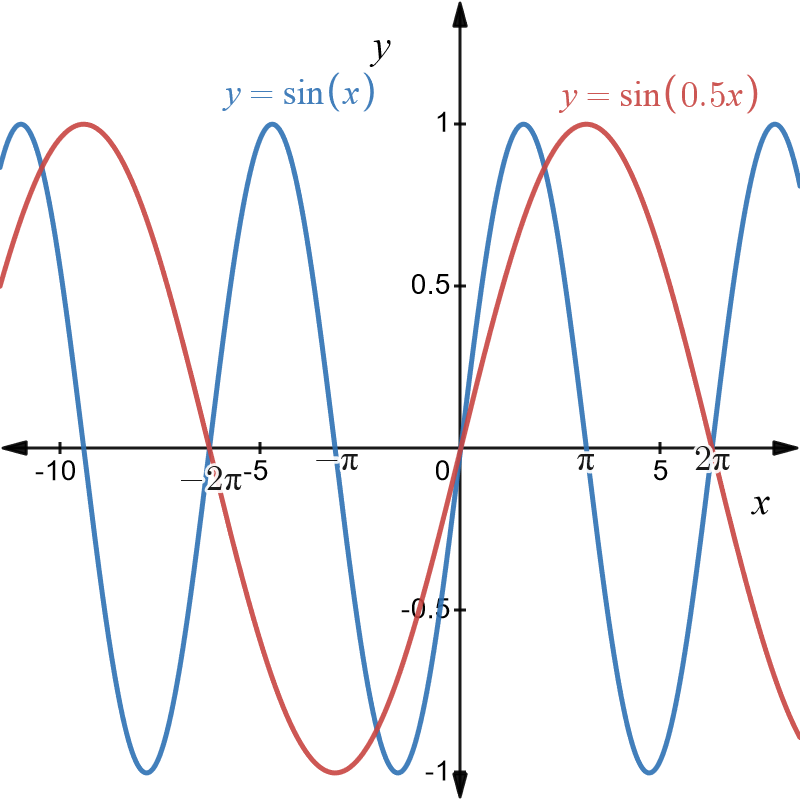
Example \(11\): Dilation of \(y=\sin\left(x\right)\) parallel to the \(x-\)axis by a factor of \(1/2\)
The graphs are shown below.
The original graph of \(y=\sin\left(x\right)\) is shown in blue. It has a period of \(2\pi.\)
The dilation \(y=\sin\left(0.5x\right)\) is shown in red and shows that the original graph is stretched parallel to the \(x-\) axis. The dilated graph has a period of \(4\pi\) which is twice that of the original graph.
Combinations of Transformations
More complicated graphs may be obtained from a basic graph by combining reflection, translation and dilation. In such cases you start with the basic graph and do the dilation first (if there is one). After this step, do translations and reflections in any order.
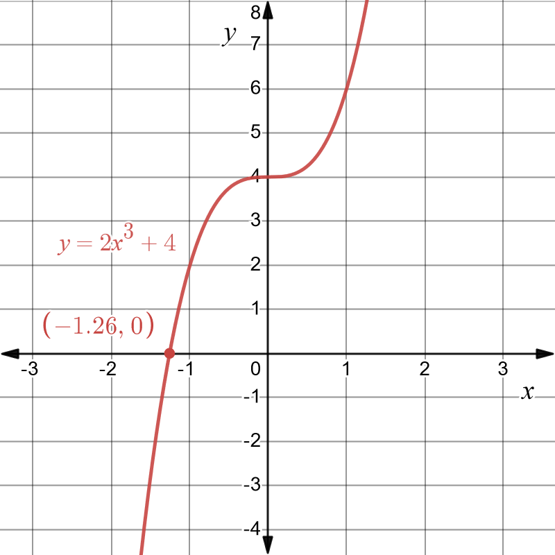
Example \(12\): Graph of \(y=2x^{3}+4\)
The basic graph is \(y=x^{3}.\) We want to transform this to \(y=2x^{3}+4.\) This involves two transformations \[\begin{align*} y & =\underbrace{\ 2\ }_{\text{Transformation1 }}x^{3}+\underbrace{\ 4\ }_{\text{Transformation 2}} \end{align*}\]
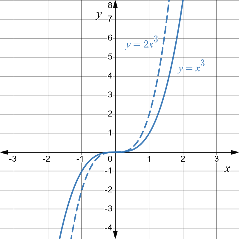
Transformation \(1\) is a dilation of 2 parallel to the \(y-\)axis. It is a stretching of the original graph parallel to the \(y-\)axis.
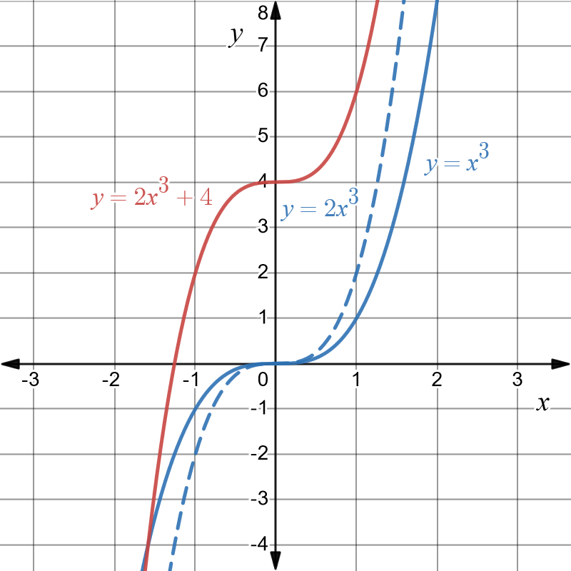
Transformation \(2\) is a translation of \(4\) units upward.
The basic graph to be transformed is \(y=x^{3}\) and is shown in blue below.
We first do the dilation on this basic graph. That is we graph \(y=2x^{3}\). This is shown as the dashed blue graph below.
Finally we do the translation of \(4\) units upwards to get the desired graph of \(y=2x^{3}+4\). This is shown in red below.
The only thing left to do is identify where the graph of \(y=2x^{3}+4\) intersects the \(x-\)axis. To do this we set \(y=0\) and solve for \(x.\) That is \[\begin{align*} 2x^{3}+4 & =0\\ 2x^{3} & =-4\\ x^{3} & =-2\\ x & =-1.26. \end{align*}\] This information can be added to get the following figure:
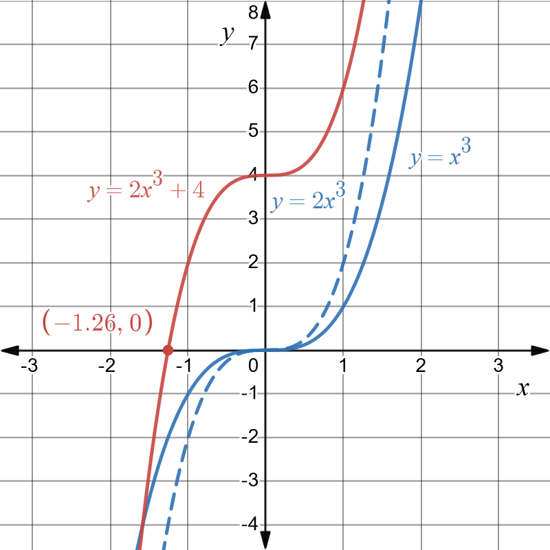
Our final answer is the red graph shown below:
Example \(13\): Graph of \(y=-\left(x+2\right)^{2}-1\)
The basic graph in this case is \(y=x^{2}.\) There are three transformations involved: \[\begin{align*} y & =\underbrace{-}_{\text{Transformation 1}}\underbrace{\left(x+2\right)^{2}}_{\text{Tranformation 2 }}\underbrace{-1}_{\text{Transformation 3}} \end{align*}\]
Transformation \(1\) is a reflection about the \(x-\)axis.
Transformation \(2\) is shift of \(y=x^{2}\) to the left by \(2\)units.
Transformation \(3\) is a shift of \(1\) unit downwards.
As there is no dilation, we are free to make the transforms on the basic graph in any order. In this example we will go from transformation \(1\) to \(3\) but the order does not matter.
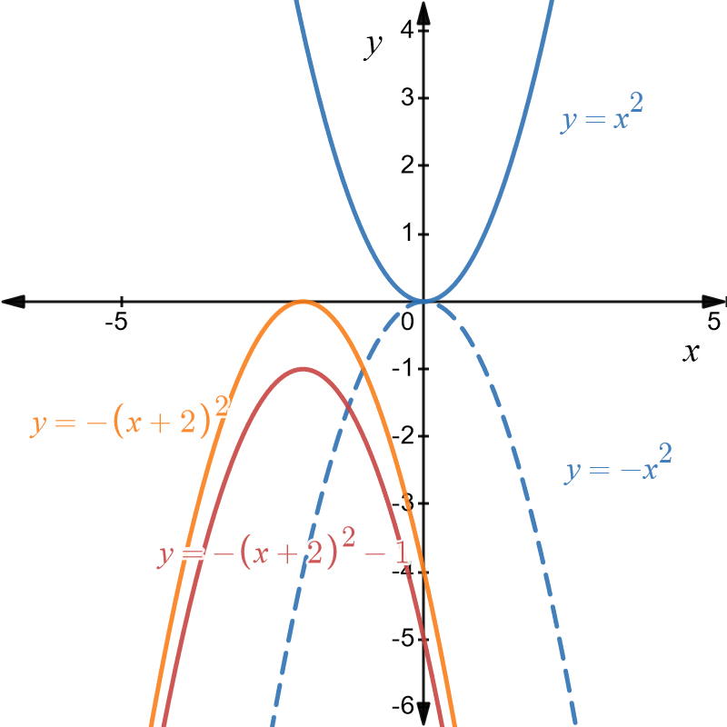
The figure below shows the basic graph \(y=x^{2}\) in blue.
Transformation \(1\) reflects this in the \(x-\)axis. This is the graph of \(y=-x^{2}\) and is shown in dashed blue below.
Transformation 2 shifts the graph of \(y=-x^{2}\), \(2\) units to the left. This is the graph of \(y=-\left(x-2\right)^{2}\) and is shown in orange.
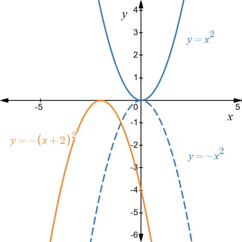
Transformation \(3\) shifts the graph of \(y=-\left(x+2\right)^{2}\) down one unit. This is the desired graph of \(y=-\left(x+2\right)^{2}-1\) and is shown below in red.
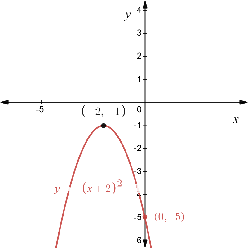
The intercept of the graph of \(y=-\left(x+2\right)^{2}-1\) appears to at \(\left(0,-5)\right)\). This can be checked by setting \(x=0:\) \[\begin{align*} y & =-\left(x+2\right)^{2}-1\\ & =-\left(0+2\right)^{2}-1\\ & =-5. \end{align*}\] The final graph of \(y=-\left(x+2\right)^{2}-1\) is shown below in red. We have marked the \(y-\)intercept at \(\left(0,-5\right)\) and the vertex at \(\left(-2,1\right).\)
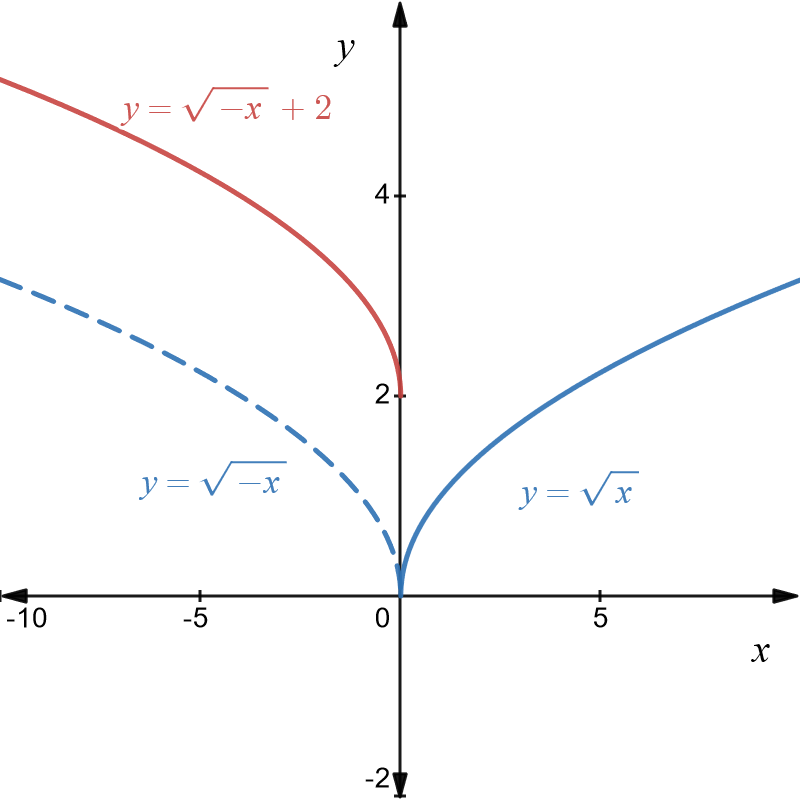
Example \(14\): Graph of \(y=\sqrt{-x}+2\)
The basic graph is of \(y=\sqrt{x}\) .
The graph of \(y=\sqrt{-x}+2\) involves two transformations: \[\begin{align*} y & =\sqrt{\underbrace{\,-x}_{\text{Transformation 1}}}+\underbrace{\,2}_{\text{Transformation 2}}. \end{align*}\]
Transformation 1 is a reflection of the graph of \(y=\sqrt{x}\) in the \(y-\)axis and is the graph of \(y=\sqrt{-x}\).
Transformation 2 is a translation of \(2\)units vertically up and gives the graph of \(y=\sqrt{x}+2\).
The graphs of \(y=\sqrt{x}\), \(y=\sqrt{-x}\), and \(y=\sqrt{-x}+2\) are shown below in blue, dashed blue and red, respectively.
Exercises
Sketch the following graphs
\(\text{1. }y=\frac{2}{x+1}\)
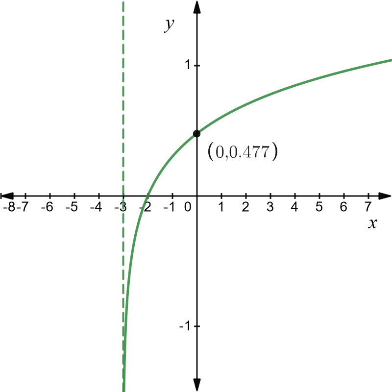
\(\text{2. }y=\log\left(x+3\right)\)
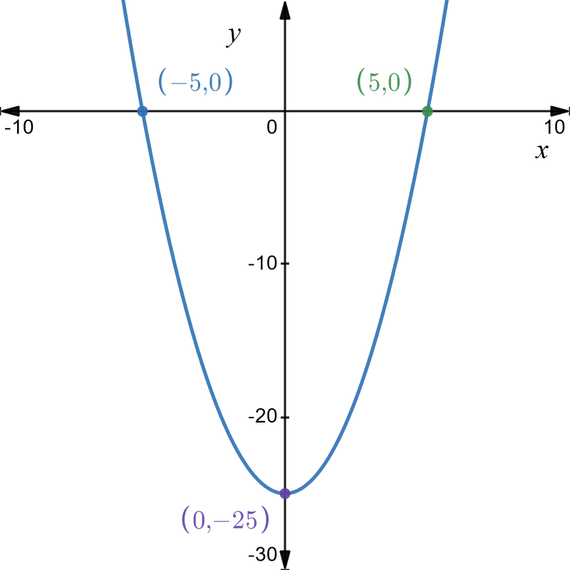
\(\text{3. }y=x^{2}-25\)
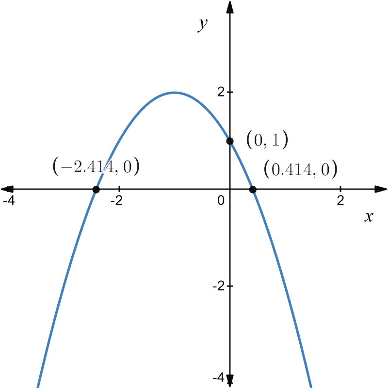
\(\text{4. }y=2-\left(x+1\right)^{2}\)
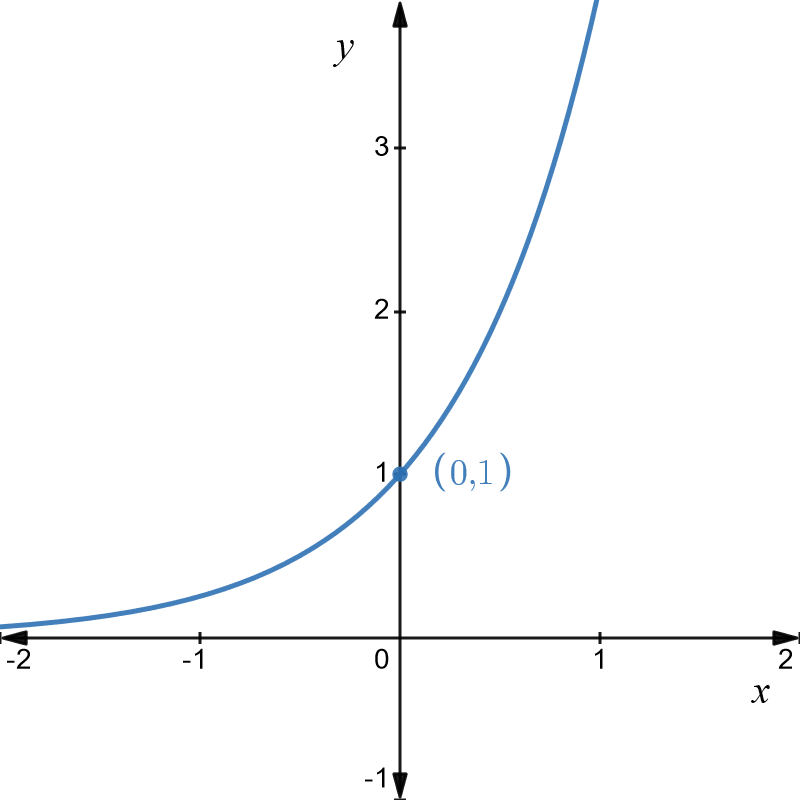
\(\text{5. }y=4^{x}\)
\(\text{6. }y=2e^{x}+1\)
Download this page, FG9 Graphs and Transformations (1029KB)
What's next... FG10 Graphs of sine and cosine functions